Scaling Laws, Carefully
📊 Level ⭐⭐⭐⭐ | 16.7KB
Scaling laws are one of the most critical empirical findings in deep learning. The observation is simple in form: the training loss decreases predictably as we scale up model size , dataset size , and compute , following a power-law curve, which appears as a straight line on a log-log plot. We can view scaling laws as a framework for describing the relationship between compute, loss, model size and data; at its core, it is about how to allocate precious compute optimally between and .
This predictability makes scaling laws highly valuable in practice. A common workflow is to fit scaling laws on a handful of small runs and then extrapolate to estimate the token and compute requirements for larger models.
| Symbol | Note |
|---|---|
| $N$ | Model size, measured in parameter count. |
| $D$ | Training dataset size, usually measured in token count. |
| $C$ | Training compute in FLOPs. As a useful approximation, $C \approx 6 N D$ (Kaplan et al. 2020), where $2 N D$ accounts for the forward pass and $4 N D$ for backpropagation. |
| $E$ | Irreducible loss |
| $L , \hat{L} \left(\right. . \left.\right)$ | Test loss / test loss prediction function; can also refer to training loss, since they are strongly correlated. |
| $\epsilon$ | Generalization error. |
Early days: ML loss predictability
The predictability of generalization error with scale had already been investigated before scaling laws became a mainstream concept.
Amari et al. (1992) derived four types of learning curves using a Bayesian approach and the annealed approximation.
- Deterministic learning algorithm, noiseless data, one unique solution: , where is some constant.
- Deterministic learning algorithm, noiseless data, multiple equivalent solutions: ; the learning is faster with each new data point, because the model only learns the optimal manifold of parameters, instead of finding the single solution point.
- Deterministic learning algorithm, noisy data: ; noises in data make learning harder.
- Stochastic learning algorithm, noisy data: ; here the irreducible loss is the residual error that a stochastic learner cannot reduce further, for example when the model runs out of capacity on large data. All four types of learning curves follow a power law:
where can be 0 and . Although their theoretical setup is based on a simplified binary classification task, it points in a useful direction for building empirical ML loss prediction models.
One of the earliest empirical studies by Hestness et al. (2017) explained the relationship between generalization error, model size and data. For a given training data size, they identified the best-fit model size via grid search and then plotted loss against training dataset size. Across four different domains in deep learning (neural machine translation, image classification, language modeling, and speech recognition), a recurring pattern was observed where:
- Generalization error scales as a power law across a set of factors (e.g. data size).
- Model improvements shift the error curve but do not seem to affect the power-law exponent.
- Interestingly, architecture changes the offset () of the power-law fit but does not change the exponent (). The slope of the power law appears to be a property of the problem domain rather than the model architecture.
- The number of model parameters needed to fit a dataset of size also scales as a power law.
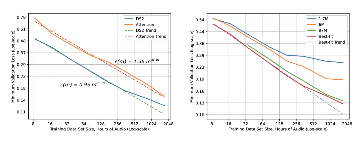
Learning curves for (Left) Deep-Speech-2 (DS2) and attention speech model and for (Right) DS2 models of various sizes. The losses of small models plateau when training data becomes large. (Image source: Hestness et al. 2017)
A conceptual illustration breaks the learning curve into three stages. In the small-data region, when there are not enough learning signals, the model performs only slightly better than random guessing. In the middle (“power-law region”), we observe a power-law relationship between loss, data, and model size. The final irreducible-error region can be attributed to factors such as noise in the data.
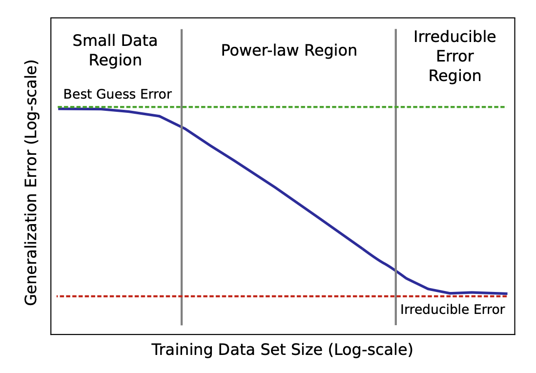
Illustration of power-law learning curve phases. (Image source: Hestness et al. 2017)
Rosenfeld et al. (2020) pushed this further by trying to model error as a joint function of both model size and data size , across a diverse set of architectures (ResNet, WRN, LSTM, Transformer) and optimizers (Adam, SGD variants). Empirically they observed that, holding one axis fixed, the error decays as a power law in the other:
which can be combined into a joint form:
where are scalar constants and is not dependent on either or .
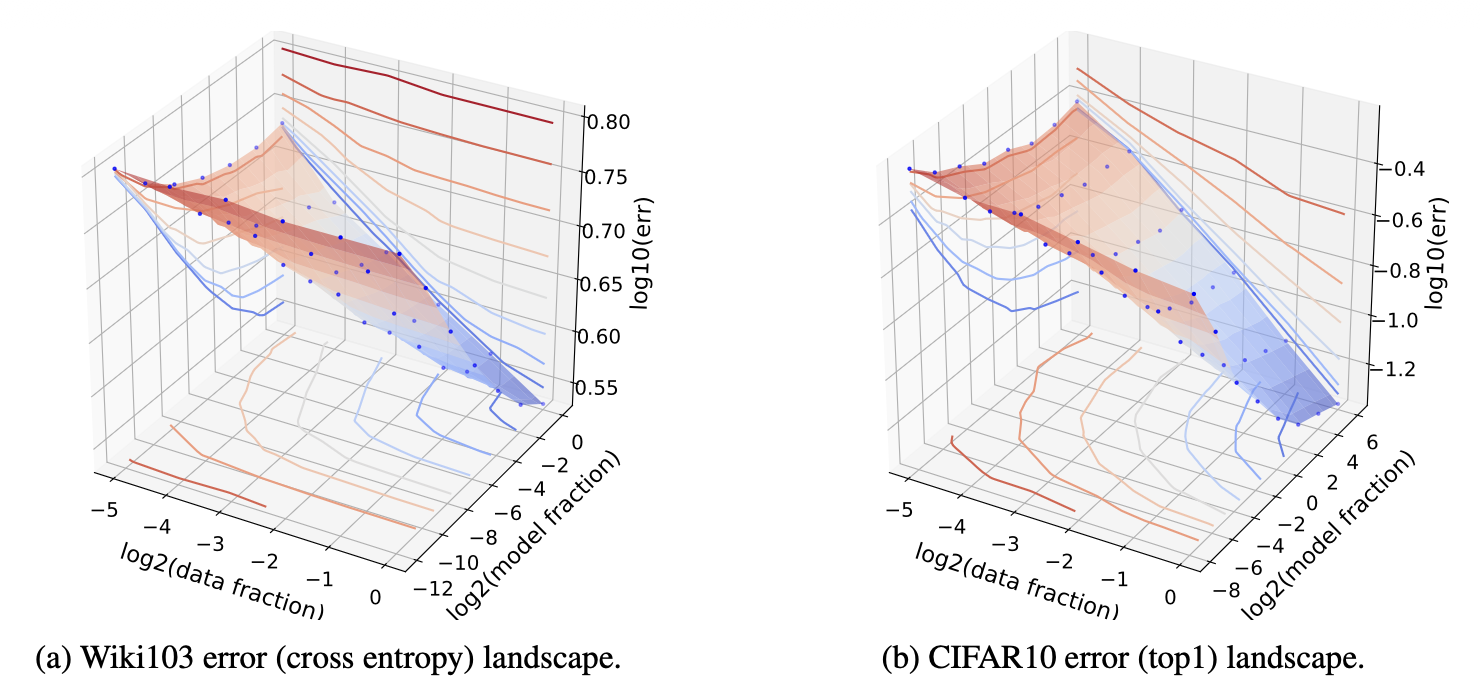
A 3D contour plot of data size, model size and generalization error in log-log-log scale. Blue dots are derived from empirical experiments and the surface is a linear interpolation between blue dots. (Image source: Rosenfeld et al. 2020)
Thus, they can build a prediction model in the form of a simple parametric function with to predict the expected loss for > certain thresholds by only training on a set of smaller training configs, < certain thresholds.
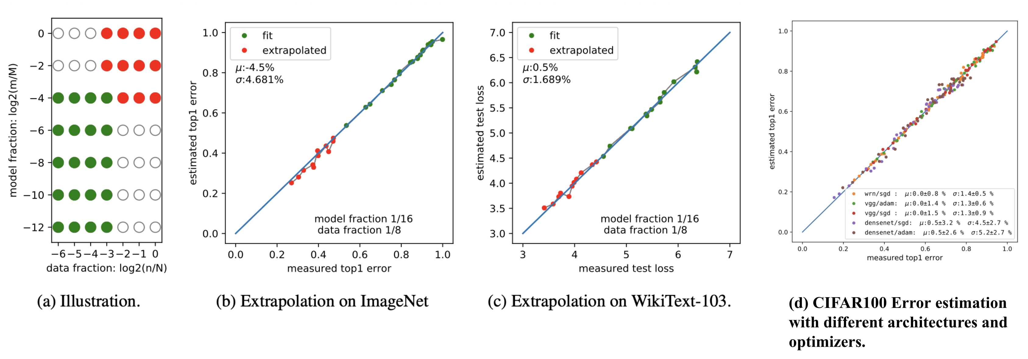
Fitting the parametric error model on small-scale configurations and extrapolating to larger model/data regimes: (a) Illustration of the experiment setup; Experiment results on (b) ImageNet, (c) WikiText-103 and (d) CIFAR100 Error estimation with three architectures (WRN, VGG, DenseNet) and two optimizers (SGD, Adam). (Image source: Rosenfeld et al. 2020)
Side note: These early works lean on
→ 原文存档
深度分析
From learning curves to parametric fits: the lineage the entity only begins to tell
The page's "Early days" section stops at the threshold of the story it sets up. Amari et al. (1992) already derived four families of learning curves — deterministic vs stochastic learners, noiseless vs noisy data — all following power laws, with the irreducible loss appearing as the floor a stochastic learner cannot push below. Hestness et al. (2017) then made the empirically decisive observation: across four domains (translation, image classification, language modeling, speech recognition), architecture shifts the offset of the power-law fit but not its exponent — the slope is a property of the problem domain, not the model. Rosenfeld et al. (2020) closed the loop by modeling error as a joint function of model size and data size, fitting a parametric surface on small configurations and extrapolating — precisely the template Chinchilla's method 3 would later reuse. Weng's side note is the kicker: classical capacity proxies like VC dimension proved too coarse for modern deep learning, and the empirical power laws were cleaner and more useful than any worst-case bound theory offered.
Kaplan vs Chinchilla: a disagreement about accounting, not about laws
The raw article's central arc is the Kaplan–Chinchilla collision. Kaplan et al. (2020) found loss scaling as a power law in parameters, data, and compute individually, and concluded model size should grow ~5.5x per 10x compute versus only ~1.8x for tokens — training a big model and stopping before convergence. Chinchilla (2022), with 400+ runs up to 16B parameters and three independent fitting methods that all agree, overturned this: for every doubling of model size, double the tokens; a 70B model on 1.4T tokens beat 280B Gopher trained on 300B. Pearce & Song (2024) reconciled the two without crowning either: Kaplan counted non-embedding parameters while Chinchilla counted total parameters, and in the small-model regime embeddings are a large enough fraction that the fitted exponent comes out locally near Kaplan's 0.73 and converges to the Chinchilla estimate as scale grows. The lesson is uncomfortable: a decade-defining "disagreement" about compute allocation was largely a parameter-accounting artifact compounded by extrapolating from small models in log-log space, where a small fit difference compounds into large predictions.
Why a power law at all: two hypotheses, no consensus
The article is candid that the shape of scaling laws has no settled explanation. Sharma & Kaplan (2020) frame language modeling as regression on a low-dimensional data manifold: more parameters partition the manifold more finely, giving the typical linear resolution a power-law form — clean in the infinite-data underfitting regime, but hampered by the fact that intrinsic dimension is genuinely hard to estimate. Michaud et al. (2023) and Brill (2024) instead assume knowledge arrives in discrete, "quantized" chunks whose frequency distribution follows a power law, so the model learns common skills first and rare ones later, producing smooth loss decay. Spectral tails, kernel eigenvalues, and phase transitions round out the alternatives — meaning the most relied-upon empirical regularity in LLM training is also one of the least theoretically grounded.
The data-limited regime: repetition has a measurable price
Classic laws assume infinite unique data; the modern constraint is the data wall. Weng stresses the token count behind any law is post-pipeline — dedup, quality filtering, decontamination, mix reweighting — so equal token counts can differ drastically in compute efficiency. On repetition, Hernandez et al. (2022) showed a double-descent where test loss first worsens then recovers as repeated data is emphasized, hurting some OOD evaluations. Muennighoff et al. (2023) quantified the remedy: a repeated token's value decays exponentially with each epoch (a learnable half-life), and up to ~4 epochs of repetition still add value — though the fit underestimates failing runs at extreme epochs. Lovelace et al. (2026) replaced the symmetric "excess model size" discount with an explicit overfitting penalty built on the capacity ratio, finding larger models are more sensitive to repetition — and that strong weight decay measurably reduces the penalty. See also domain data repetition in LLM pretraining for the domain-mix angle.
Fitting is fragile: replication as a service
The closing section is the article's most practical warning. Because a law is fit on small affordable runs and extrapolated orders of magnitude beyond them, seemingly trivial procedural choices — parameter counting, precision rounding, summing vs averaging loss — can swing predictions wildly, while the fit silently assumes architecture, optimizer, LR schedule, batch ramp, data mix, and tokenizer are held constant and well-tuned. Besiroglu et al. (2024) proved this is not hypothetical: re-extracting Chinchilla method 3's data, they found averaging (rather than summing) Huber loss caused premature L-BFGS termination with implausibly narrow confidence intervals, and 2-digit rounding made the derived frontier look worse than it was. The article's toy simulation then demonstrates the failure modes live: loss rounding, milli-loss noise, and fit-region choice each produce different "laws".
实践启示
1. Treat small-run extrapolation as a hypothesis test, not a budget forecast
The fit-on-small-runs workflow is only as good as its assumptions. Because predictions are extrapolated across orders of magnitude in log-log space, any procedural artifact in the small runs is amplified, not averaged out. Before committing a large training budget, replicate the fit with at least two independent methodological choices and treat divergence between them as the real error bar. The scaling laws concept page tracks the ongoing refinements.
2. Fix the accounting before trusting the fit
Decide and document what counts as a parameter (embedding in or out), how loss is aggregated, and what precision is kept — before fitting. The Kaplan–Chinchilla dispute was substantially an embedding-accounting mismatch, and the Chinchilla method 3 replication found a loss-aggregation bug that early-stopped the optimizer.
3. Budget data quality as compute, not as a preprocessing detail
Two datasets with identical token counts can yield drastically different compute efficiency depending on dedup, filtering, and mixture quality. When a run underperforms its scaling-law prediction, audit the data pipeline before blaming the law or the architecture — the law was fit on data with a quality profile your run may not share.
4. In the data-constrained era, repeat deliberately and watch model size
Repetition is not a failure state: token value decays exponentially but stays positive for roughly the first ~4 epochs, while over-parameterized models overfit repeats faster. Under a fixed unique-token budget, prefer more epochs on a right-sized model over a larger model, tune weight decay to suppress the repetition penalty, and treat model size scaling trajectories as bounded by data, not ambition. See also LLM pretraining vs SFT for where pretraining loss gains actually transfer downstream.
5. Don't over-index on architecture — but do hold it fixed mid-experiment
Hestness's finding that architecture moves the offset but not the exponent, echoed by Kaplan's "architectural details matter less than scale", suggests effort spent micro-tuning width or aspect ratio buys less than data or scale. The flip side: scaling-law fits are only valid under a frozen architecture/data-mix, so any mid-campaign architecture or tokenizer change invalidates the extrapolation you were relying on.
关联
- 相关概念: Harness Engineering